Page History

...

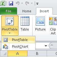
1. On a sheet, different than the sheet with the data markers, select the cell where you would like to insert the pivot table.
   #
   
2. Go to Insert > PivotTable on the Excel ribbon
   \\\
   
   
   
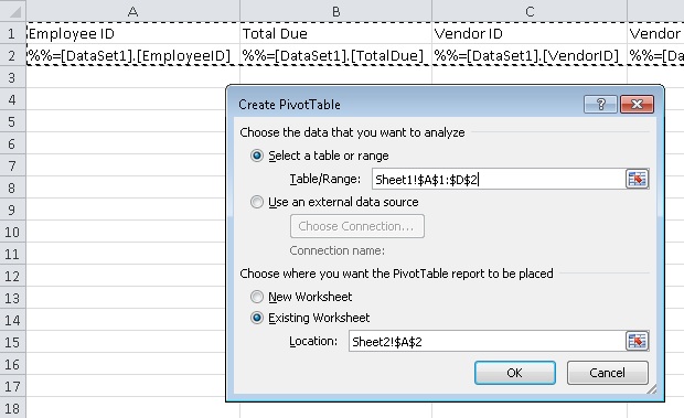
3. # When prompted to select data, navigate to the sheet with the data markers. Select the header row and the data marker row. Click OK when finished.
   \\\
   
   #
   
4. This will insert a blank PivotTable into the second worksheet.
   \\\
   
   
   
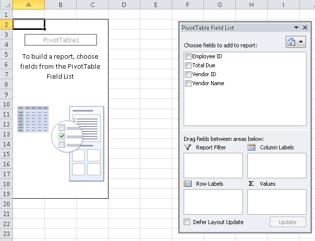
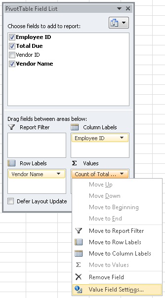
5. # Drag VendorName into the Row Labels section and EmployeeID into the Column Labels section. Drag TotalDue into the Values section.
   \\\
   
   #
   
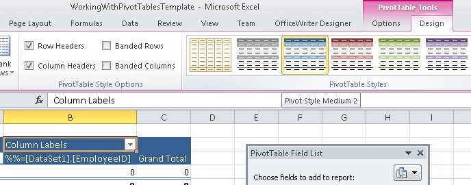
6. In the Excel ribbon, go to Design and select a style to apply to the PivotTable.
   \\\
   
   
   

You've added a PivotTable to your report, but there are a few settings that need to be changed before we're done.

Field Settings and PivotTable Options

...

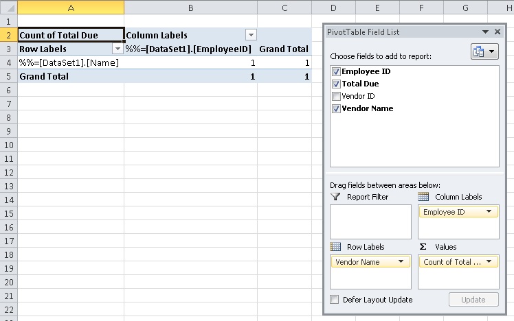
1. You will note that the formula used to aggregate the TotalDue field is currently set to Count. This is because the only data in the data source is a data marker, which is a string. Right click the TotalDue field and select Value Field Settings.
   \\\
   
   #
   
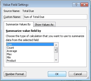
2. Switch the summarize formula to be Sum instead of Count. Click OK when finished.
   \\\
   

PivotTable Options

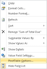
1. Right click on the PivotTable go select PivotTable Options
   \\\
   
   #
   
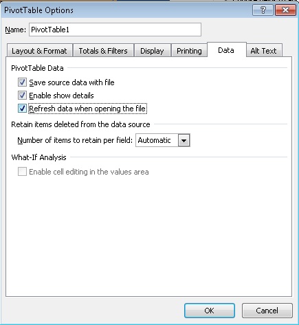
2. Go to the Data tab.
   
   
3. # To make sure that the new imported data is pulled into the PivotTable when you open the rendered report, you have to set the PivotTable to Refresh data when opening the file.
   
   If you don't do this, your PivotTable will look exactly the same as it does in the template until the PivotTable is refreshed.
   \\\
   
   
   
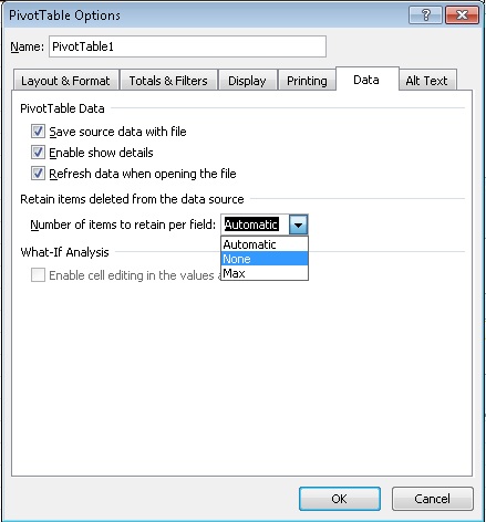
4. # Under the Retain items deleted from the data source you will see a Number of items to retain per field drop-down. Select None from the dropdown.
   
   If you don't, the data markers that are currently in your data source will be carried over to the output file. The data markers will appear in the PivotTable label filters.
   \\\
   
   #
   
5. Click OK when finished.

You are now done setting up the PivotTable in your report template.

...

1. From the export option drop-down list, choose Excel designed by Officewriter.
   
   
2. # You will be prompted to save or open the output file. If your report contains a PivotTable AND you are using Internet Explorer 8 or earlier, you MUST select Save. After it saves to disk, then you may select Open to view it.

...