Page History

...

1. On a sheet, different than the sheet with the data markers, select the cell where you would like to place the PivotTable for the PivotChart. A PivotChart is powered by an underlying PivotTable, so you will need to create a PivotTable at the same time as the PivotChart.
   #
   
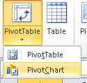
2. Go to Insert > Pivot Chart on the Excel ribbon.
   \\\
   
   
   
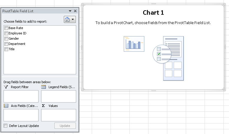
3. # This will insert a blank PivotChart and PivotTable into the worksheet. You may notice that the labels in the Pivot Fields box have changed to reflect that we are designing for a PivotChart (e.g. Row labels >> Axis labels)
   
   
   #
   
4. Drag the Department pivot field into the Report Filter section. Drag Title into Axis Fields, Gender into Legend Fields, and Base Rate into Values. When you are done you should have a PivotChart that looks like this:
   !setup_pivotchart.png!
   #
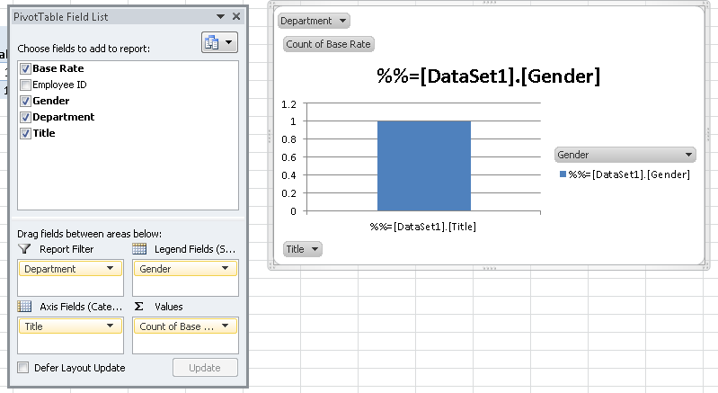   Image Added
   
   
5. The default PivotChart type is a basic column chart. To change the chart type, select the PivotChart and then go to Change Chart Type in the PivotChart tools ribbon (which is available when a PivotChart is selected).
   !changecharttype.png!
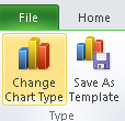   Image Added
   #
   
6. Let's change the chart type to 3D Clustered Column.
   !switchcharttype.png!
   \
   
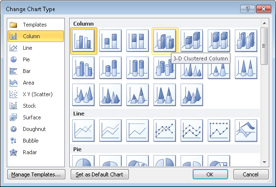   Image Added
   
   

Now that you have a basic PivotChart in your report, you will need to make some changes to the field settings and PivotTable options before the template is finished.

Field Settings

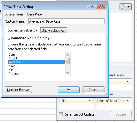
Just as we did for the PivotTable in Working with PivotTables, we will want to change the Values computation from Count to something more useful.

Right click on Count of Base Rate in the Values section in the Pivot Fields menu and switch the calculation to Average.
\

Refreshing the Data

We mentioned earlier that PivotCharts are powered by underlying PivotTables. To make sure that the new data is pulled into the PivotTable (and therefore the PivotChart), the data source needs to refresh when the workbook opens.

1. Right click the PivotTable or PivotChart and select PivotTable Options from the drop-down.
   #
   
2. Go to the Data tab
   
   
3. # Check off Refresh data when opening the file
   
   
4. # To avoid pulling the data markers into the filters of the final report, select None from the Number of items to retain per field dropdown.
   !pivottable_options.png!
   #
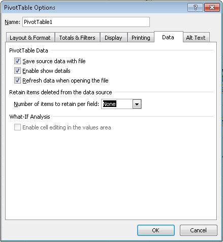   Image Added
   
   
5. Click OK when you are finished.

Your PivotChart is now finished and should look like this:
!final_template_chart.png!
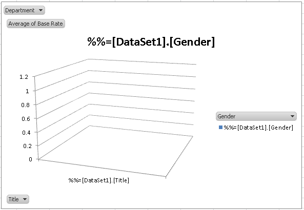Image Added

Viewing the PivotChart

...

1. From the export option drop-down list, choose Excel designed by Officewriter.
   
   
2. # You will be prompted to save or open. If your report contains a PivotTable/PivotChart AND you are using Internet Explorer 8 or earlier, you MUST select Save. After it saves to disk, then you may select Open to view it.
   \
   This is because of an issue with how Internet Explorer caches temporary internet files. If you are using any other browser or Internet Explorer 9 or later, this issue does not occur and you can open the file directly.