...

Since the formulas are native Excel functionality, we will only be modifying the template file. There are no changes to the code from Part 1.

Working with Formulas

...

Combining Data Markers with Text

We start with the template file as it was at the end of Part 1:

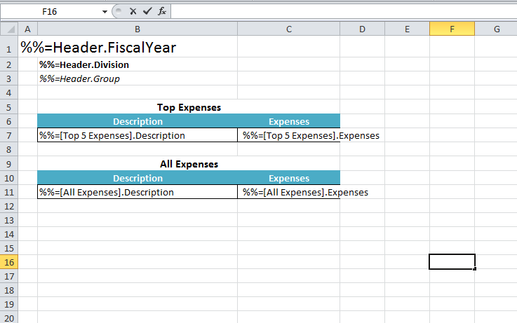
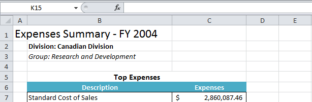
Right now, the header is set up just to display the values for FiscalYear, Division, and Group. Let's say we want to change the labels to "Expenses Summary - <Fiscal Year>", "Division: <Division>", "Group: <Group>". Data markers must be the only content a cell, they cannot be combined with other text. To get around this, you need to build the text or formula with a reference to the cell the data marker occupies.

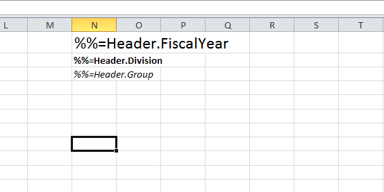
1. Move the data markers for %%=Header.FiscalYear, %%=Header.Division, %%=Header.Group to a column off to the right, say Column N.

Image Added

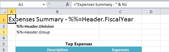
2. In A1, replace %%=Header.FiscalYear with a formula that builds the desired string with the formula ="Expenses Summary - " & N1.

Image Added

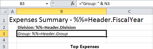
3. In B2 and B3, replace %%=Header.Division and %%=Header.Group with similar formulas: ="Division: " & N2, ="Group: " & N3.

Image Added

4. Hide column N so the extra data markers won't be visible.

5. Run the code.
In the output you will see the text combined with the values of the data markers:

Image Added

Using Inline Formulas

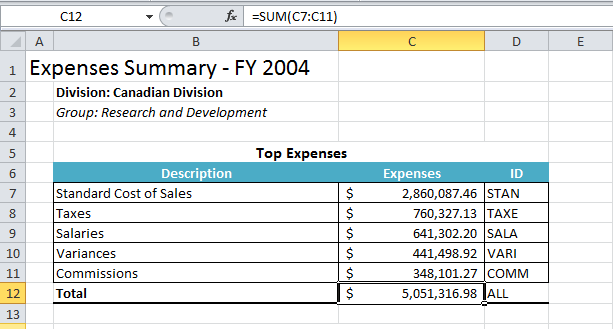
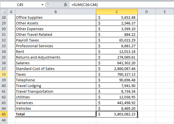
If a formula references a data marker row, ExcelWriter will update the formula to reflect that multiple rows are being inserted. In this section, we'll briefly cover how ExcelWriter handles formulas that are on the data marker row.

...

You will see that the formulas have been stretched and updated as described above.

Combining Data Markers with Text

Right now, the header is set up just to display the values for FiscalYear, Division, and Group. Let's say we want to change the labels to "Expenses Summary - <Fiscal Year>", "Division: <Division>", "Group: <Group>". Data markers must be the only content a cell, they cannot be combined with other text. To get around this, you need to build the text or formula with a reference to the cell the data marker occupies.

1. Move the data markers for %%=Header.FiscalYear, %%=Header.Division, %%=Header.Group to a column off to the right, say Column N.

Image Removed

2. In A1, replace %%=Header.FiscalYear with a formula that builds the desired string with the formula ="Expenses Summary - " & N1.

Image Removed

3. In B2 and B3, replace %%=Header.Division and %%=Header.Group with similar formulas: ="Division: " & N2, ="Group: " & N3.

Image Removed

4. Hide column N so the extra data markers won't be visible.

5. Run the code.
In the output you will see the text combined with the values of the data markers:

Image Removed

Final Code

using SoftArtisans.OfficeWriter.ExcelWriter;
...
ExcelTemplate XLT = new ExcelTemplate();

XLT.Open(Page.MapPath("//templates//part1_template.xlsx"));

DataBindingProperties dataProps = XLT.CreateDataBindingProperties();

object[] valuesArray = { "FY 2004", "Canadian Division", "Research and Development" };
string[] columnNamesArray = { "FiscalYear", "Division", "Group" };

XLT.BindRowData(valuesArray, columnNamesArray, "Header", dataProps);

DataTable dtTop5 = GetCSVData(Page.MapPath("//data//Part1_Top5Expenses.csv"));
DataTable dtAll = GetCSVData(Page.MapPath("//data//Part1_AllExpenses.csv"));

XLT.BindData(dtTop5, "Top 5 Expenses", dataProps);
XLT.BindData(dtAll, "All Expenses", dataProps);

XLT.Process();

XLT.Save(Page.Response, "Part1_Output.xlsx", false);

...