
.
...
1. Select the 9 cells in the percentage grid at the top of the worksheet (C4:E6).
2. Right click and select "Format Cells..."
3. Select "Percentage" on the Number tab.
4. Click OK
5. Select cells C12:F12, C17:F17, and C22:D22.
6. In the top tool bar, under the 'Number' tab, click the "$" to apply the currency format.
...
As ExcelTemplate populates the worksheet, the number format will be copied to all the new rows of data that are inserted where the data markers are.
The next step is setting up the table. Add a header and label the rows and columns to end up with a complete table: 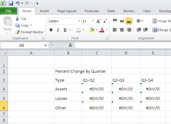
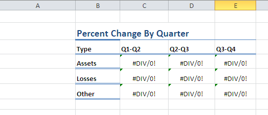
Once the table is complete, add styles.
1.Select "Percent Change by Quarter" and set it to "Heading 1." Heading 1 is found in the named styles list, on the "Home" tab of the ribbon.
2. Select the header row (B3:E3) and set it to "Total" in the named styles menu.
3. Select the row labels (B4:B6) and set that to "Total."
You should now have this:
4. Select the area of B3:E6, and apply a consistent border:
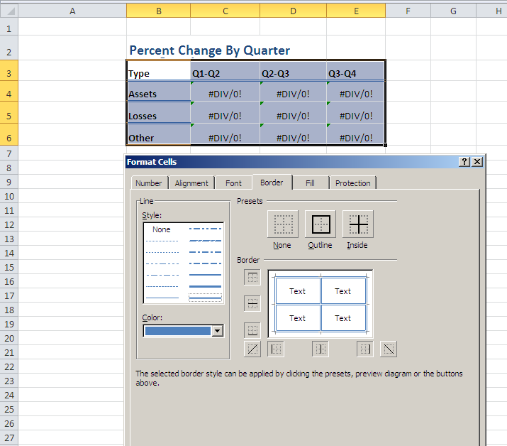
5. Now select B2:E2 and apply a bottom border in dark blue.
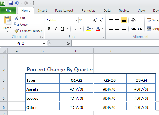
The template should look like this:
...
ExcelTemplate will preserve existing conditional formatting. If the conditional format includes a formula, that formula will also be updated as new rows are inserted into the file.
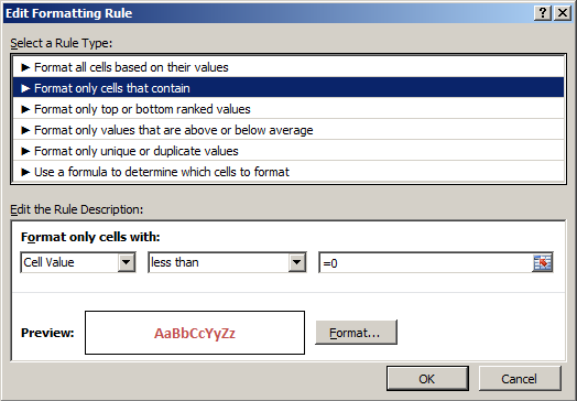
In this case, the conditional formatting will be applied to the 'percent table' and it format negative numbers to be bold and red.
1. On the "Home" tab in Excel, click on "Conditional Formatting"
...
5. Click OK to save the rule. 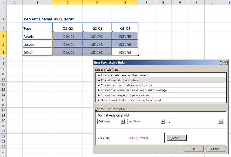
...