
.
...
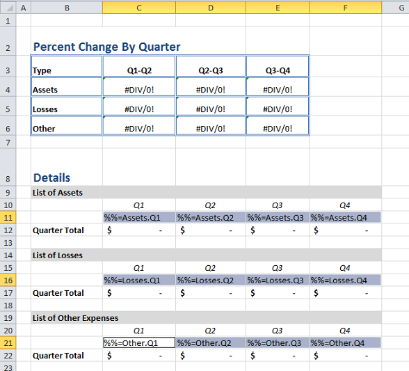
The bottom of the worksheet has a section for the data that will be imported. Each section has a total row summing all of the values for the section. This formula will expand as ExcelTemplate imports data.
This sub-report makes use of a data sheet. This is where the data markers will go. It should look something like this: 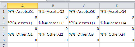
The alternating rows (highlighting added for demonstration) contain the SUM Excel formula. The formula is visible in the function bar below: 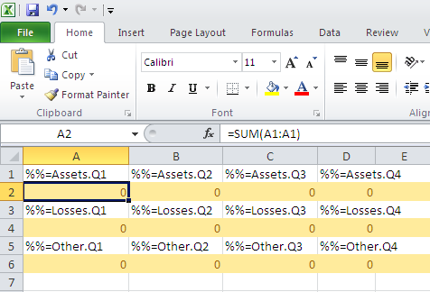
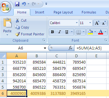
The sum formula is a standard Excel function, which gets updated when ExcelWriter populates the file with data. When the data is populated, the A1:A1 reference gets updated to include all the rows of data. The result should be something like this (highlighting added for demonstration):
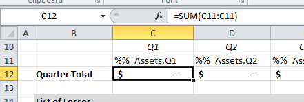
The next step is adding references to the data sheet. This example references the "SUM" formulas on the data sheet. These sums are added to a percent change equation. This will result in a template resembling the following: 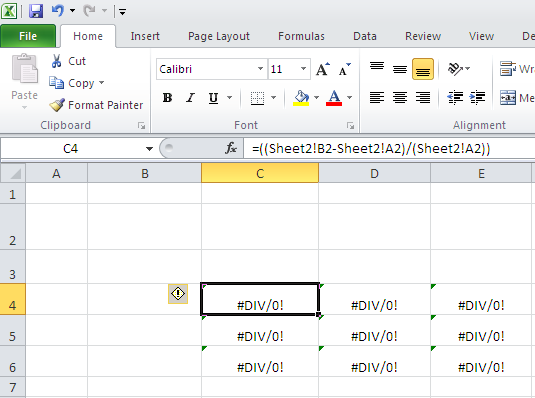
Note the formula in the formula bar, "Sheet2" is the data sheet.
| Info | ||
|---|---|---|
| ||
In this example, the sum rows alternate on the data sheet. If you stretch a formula, you'll have to update the references to skip every other row. |
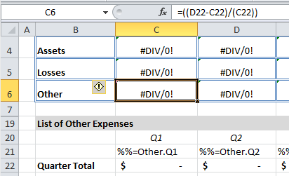
The formula we are using shows percent change. It is set up like this: At the top is a grid that calculates the percent in change between each quarter, based on the asset, loss, and other totals. The formulas are set up as "=(Sheet2!B2-Sheet2!A2)/(Sheet2!A2)" for each cell in the grid.
The value returned by the percent change equation should be displayed as a percentage. The table cells all have to be formatted.This section will cover how to add number formatting and the expected behavior for ExcelTemplate as it imports data.
1. Select all cellsthe 9 cells in the percentage grid at the top of the worksheet (C4:E6).
2. Right click and select "Format Cells..."
3. Select "Percentage" on the Number tab.
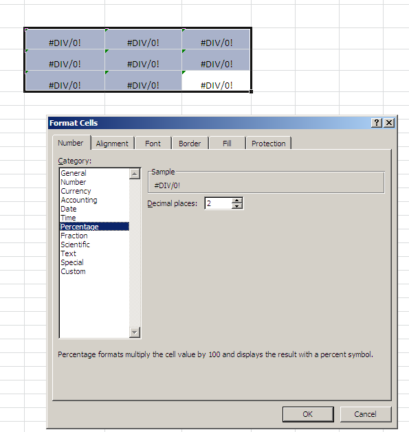
4. Click OK
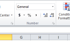
5. Select cells C12:F12, C17:F17, and C22:D22.
6. In the top tool bar, under the 'Number' tab, click the "$" to apply the currency format.
So far the number formats have been applied to cells that only contain formulas, but number formats also work with cells that contain data markers.
1. Select cells C11:F11, C16:F16, C21:F21.
2. At the top bar, click the "$" to apply the currency format.
As ExcelTemplate populates the worksheet, the number format will be copied to all the new rows of data that are inserted where the data markers are.
The next step is setting up the table. Add a header and label the rows and columns to end up with a complete table: 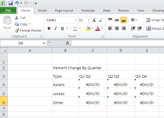
Once the table is complete, add styles.
...