
.
...
Here is the starting template: 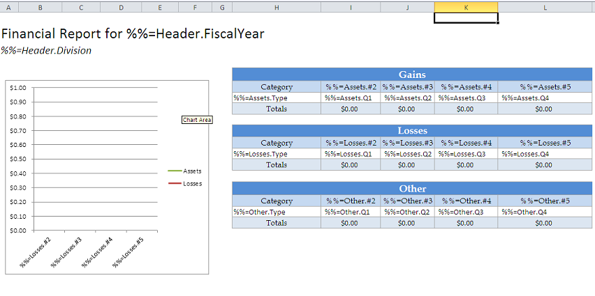
The next few steps will demonstrate adding show the process of adding data marker modifiers.
ExcelTemplate supports the use of ordinal numbering based on data source column. Instead of binding to "%%=Assets.Q1" the data marker can bind to the second column in the Assets data set with the syntax "%%=Assets.#2." Note that the hash (#) indicates ordinal syntax. An example is below:
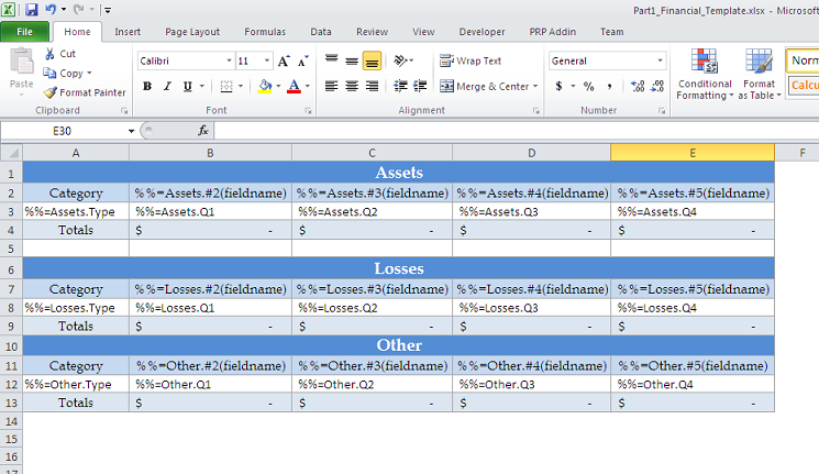
This template uses two different data marker modifiers - fieldname and optional. Modifiers are added in parentheses at the end of a data marker. They alter the binding behavior of the data marker.
The fieldname modifier shows the fieldname of the column being bound. It will not bind any additional data. It is used like thisThe syntax is as follows:
The optional modifier allows that data marker to be ignored on data binding. The optional modifier allows you to bind data if the column might be empty. It is used like this:
...
The optional modifier allows the data marker to be ignored if there is no data corresponding with that column.
...
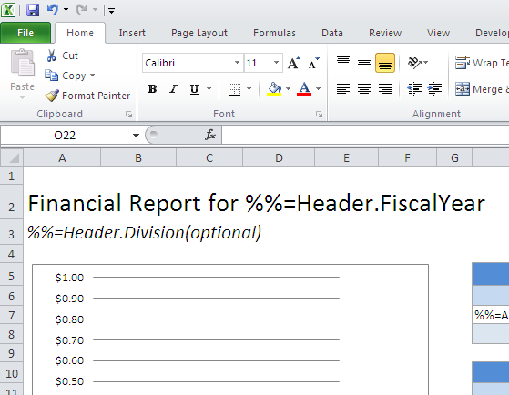
This is just an ignore - the column itself will still exist, but the data marker will be skipped. Here is a usage example:
In the above, the "Division" column will be ignored if no division is present in the data.
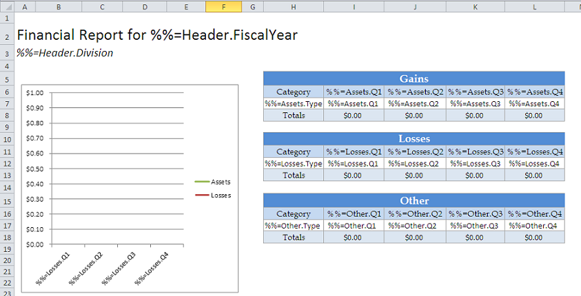
After the modifiers are added, the template should resemble this: 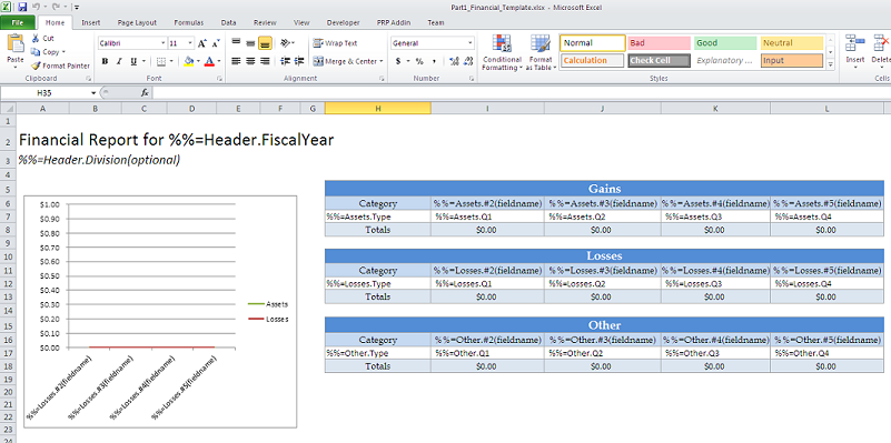
| Warning |
|---|
Move to part 2 |
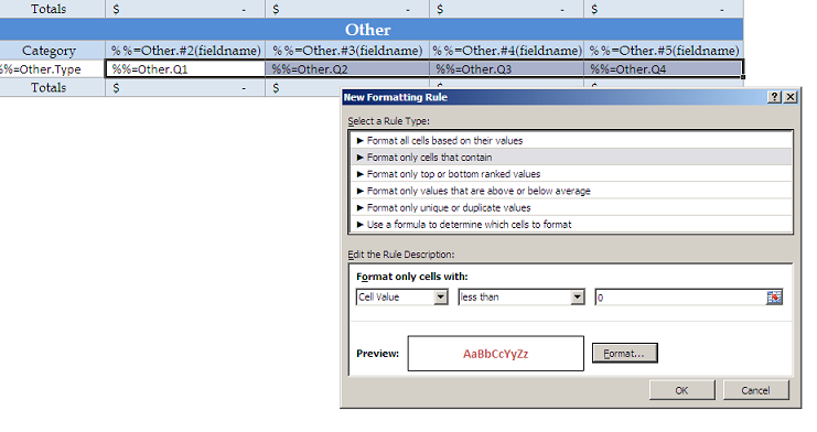
ExcelTemplate will persist conditional formatting in a template. In this tutorial, conditional formatting is applied to the "Other" table. It sets negative numbers to be red and bold.
1. On the "Home" tab in Excel, click on "Conditional Formatting"
2. Select "New Rule..."
3. In this tutorial the condition type is "Format only cells that contain..." The rule is "Cell value less than 0"
4. Click on "Format..." Set the text to be dark red. Set the typeface to be bold.
5. Click OK to save the rule.
...