Background
A PivotTable is an interactive table that summarizes data to present it in a meaningful way. You can rotate a PivotTable's rows and columns to see different summaries of the source data, or drill down to show details. By displaying different views of data, PivotTable reports allow you to easily compare data, see patterns and relationships, and analyze trends.
...
With OfficeWriter, you design your PivotTable only once at report design-time. Each time you run the report, OfficeWriter will export the report to Excel and plug the data into the PivotTable. In this section we will explore using PivotTables in a report created with OfficeWriter Designer.
Setup
Step 1. Add Data Markers to Your Workbook
- Open Microsoft Excel and create a new workbook.
# Click Add Query on the OfficeWriter toolbar.
# Follow steps 2-11 of Create a Database Query.
# In the Add Tables dialog box, find the Purchasing.PurchaseOrderHeader table in the list and select Add. Click Close.
# In Microsoft Query, drag the following fields to the query:EmployeeID, TotalDue, and VendorID.
!xlw_Pivot1.jpg!
# Add the Purchasing.Vendor table and its Name field to the query. You should see that the two tables are related by the VendorID field.
!xlw_Pivot2.jpg!
# From the File menu, select Return to OfficeWriter Designer.
# Add the fields - as data markers - and a header row to your report, as shown.
!xlw_Pivot3.jpg!
# Publish the report.
# Click View on the OfficeWriter toolbar to see the populated report.
# Click Close Report View to return to the report template.
Step 2. Create a PivotTable
- With your mouse, highlight both the header row and the row containing your fields.
# Open Excel's Data menu and select PivotTable and Pivot Chart Report to open the PivotTable Wizard.
# Select Microsoft Office Excel list or database from the top section and PivotTable from the bottom section and click Next.
# Since you highlighted the header and field rows of your report, the Step 2 screen should already contain the cell range to use. Click Next.
# Select New Worksheet and click Finish. You should now have an empty PivotTable in your worksheet, as shown.
!xlw_Pivot4.jpg!
# Click the Vendor Name field from the field list box and drag it to where it says Drop Row Fields Here.
# Click and drag the Employee ID field to where it says Drop Column Fields Here.
# Click and drag Total to where it says Drop Data Items Here. Your PivotTable should look like this:
!xlw_Pivot5.jpg!
# By default, this will give us a count of rows for each vendor/employee combination. However, for our example, we want a sum of the totals for each vendor/employee. So, on the PivotTable where it says Count of Total, right-click and select Field Settings. Under Summarize by, change Count to Sum and click Ok. Your PivotTable should now look like this:
!xlw_Pivot6.jpg!
\ Data Placeholders
When the report is executed, the data markers that you created in Step 1 will be replaced with values from the database. To ensure that the PivotTable is constructed properly, you must replace the data markers with placeholder data - any data that will be of the same format as the real output data. For example, if the field is numeric, such as our EmployeeID field, we may use a zero or any other number. If the field is a character field, such as the Name field, we need to use a character placeholder. For our example, we will use the word 'none' for Name and a zero for EmployeeID.
- Under the Vendor Name label, replace =%%Query1.Name with none.
# Under the Employee ID label, replace =%%Query1.EmployeeID with 0.
!xlw_Pivot7.jpg!
| Note |
|---|
When you insert placeholder data, never use a real value. For example, if you are displaying a city name, don't use 'Boston' for the placeholder data. The results returned for 'Boston', in that case, may not behave as expected. The same holds true for numeric data. Try to find a value that will never actually be in the query's result set. |
Refreshing the Data
There is one more thing to do before trying our PivotTable. Right-click on the PivotTable and select Table Options. Near the bottom of the left column, make sure Refresh on Open is checked. If you do not check this, when the report is viewed, your PivotTable will be empty.
 Image Removed
| Note |
|---|
The following example uses the AdventureWorks sample database that ships with SQL Server Reporting Services 2005. It is assumed that you already know how to set up a report in Excel using OfficeWriter Designer. If you do not know how to do this, see |
...
This query returns company purchase data from the AdventureWorks database, sorted by Vendor ID and Employee ID. This is the data that will be used in this report.
| Code Block |
|---|
|
SELECT PurchaseOrderHeader.EmployeeID,
      PurchaseOrderHeader.TotalDue,
      PurchaseOrderHeader.VendorID,
      Vendor.Name
FROM AdventureWorks.Purchasing.PurchaseOrderHeader
JOIN AdventureWorks.Purchasing.Vendor
ON Vendor.VendorID = PurchaseOrderHeader.VendorID
ORDER BY PurchaseOrderHeader.VendorID, EmployeeID
|
Below is a screenshot of an Excel template with data markers that will be populated with the data from the ahove query.
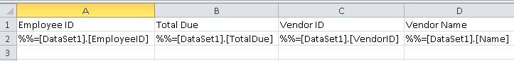 Image Added
After running the report, the imported data looks like this:
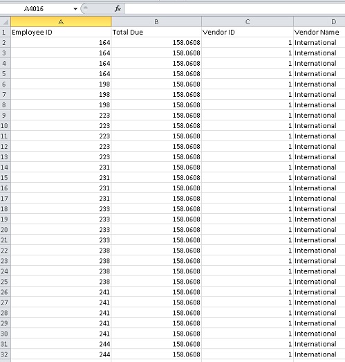 Image Added
Creating a PivotTable
- On a sheet, different than the sheet with the data markers, select the cell where you would like to insert the pivot table.
# Go to Insert > PivotTable on the Excel ribbon
\\\ 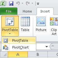 Image Added
# When prompted to select data, navigate to the sheet with the data markers. Select the header row and the data marker row. Click OK when finished.
\\\ 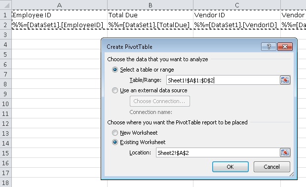 Image Added
# This will insert a blank PivotTable into the second worksheet.
\\\ 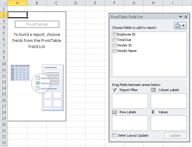 Image Added
# Drag VendorName into the Row Labels section and EmployeeID into the Column Labels section. Drag TotalDue into the Values section.
\\\ 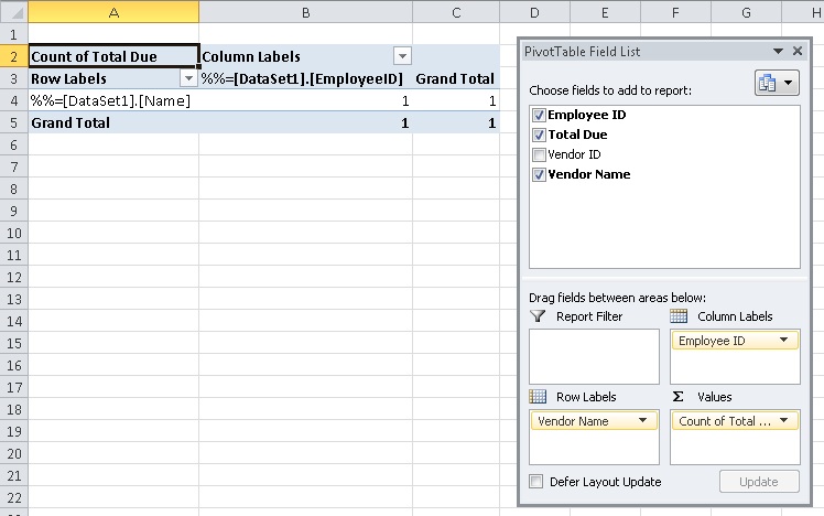 Image Added
# In the Excel ribbon, go to Design and select a style to apply to the PivotTable.
\\\ 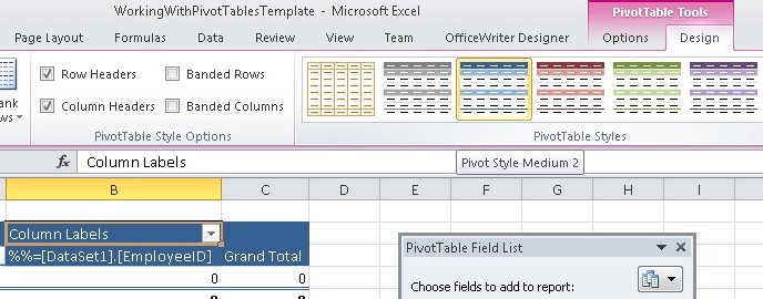 Image Added
You've added a PivotTable to your report, but there are a few settings that need to be changed before we're done.
Field Settings and PivotTable Options
Field Settings
- You will note that the formula used to aggregate the TotalDue field is currently set to Count. This is because the only data in the data source is a data marker, which is a string. Right click the TotalDue field and select Value Field Settings.
\\\ 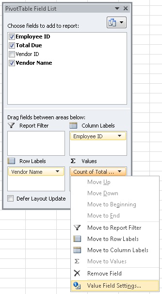 Image Added
# Switch the summarize formula to be Sum instead of Count. Click OK when finished.
\\\ 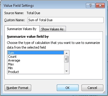 Image Added
PivotTable Options
- Right click on the PivotTable go select PivotTable Options
\\\ 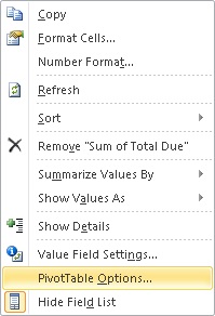 Image Added
# Go to the Data tab.
# To make sure that the new imported data is pulled into the PivotTable when you open the rendered report, you have to set the PivotTable to Refresh data when opening the file.
If you don't do this, your PivotTable will look exactly the same as it does in the template until the PivotTable is refreshed.
\\\ 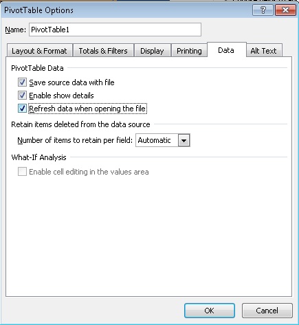 Image Added
# Under the Retain items deleted from the data source you will see a Number of items to retain per field drop-down. Select None from the dropdown.
If you don't, the data markers that are currently in your data source will be carried over to the output file. The data markers will appear in the PivotTable label filters.
\\\ 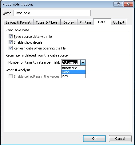 Image Added
# Click OK when finished.
You are now done setting up the PivotTable in your report template.
Viewing the PivotTable
Publish, and View your report. Notice that on the first sheet, your data columns display the correct data.
Image RemovedImage Added
Now look at the sheet containing your PivotTable. You should find the EmployeeID numbers across the top and all the vendor names along the left column. Each cell will contain the sum for each vendor/employee combination.
Image Removed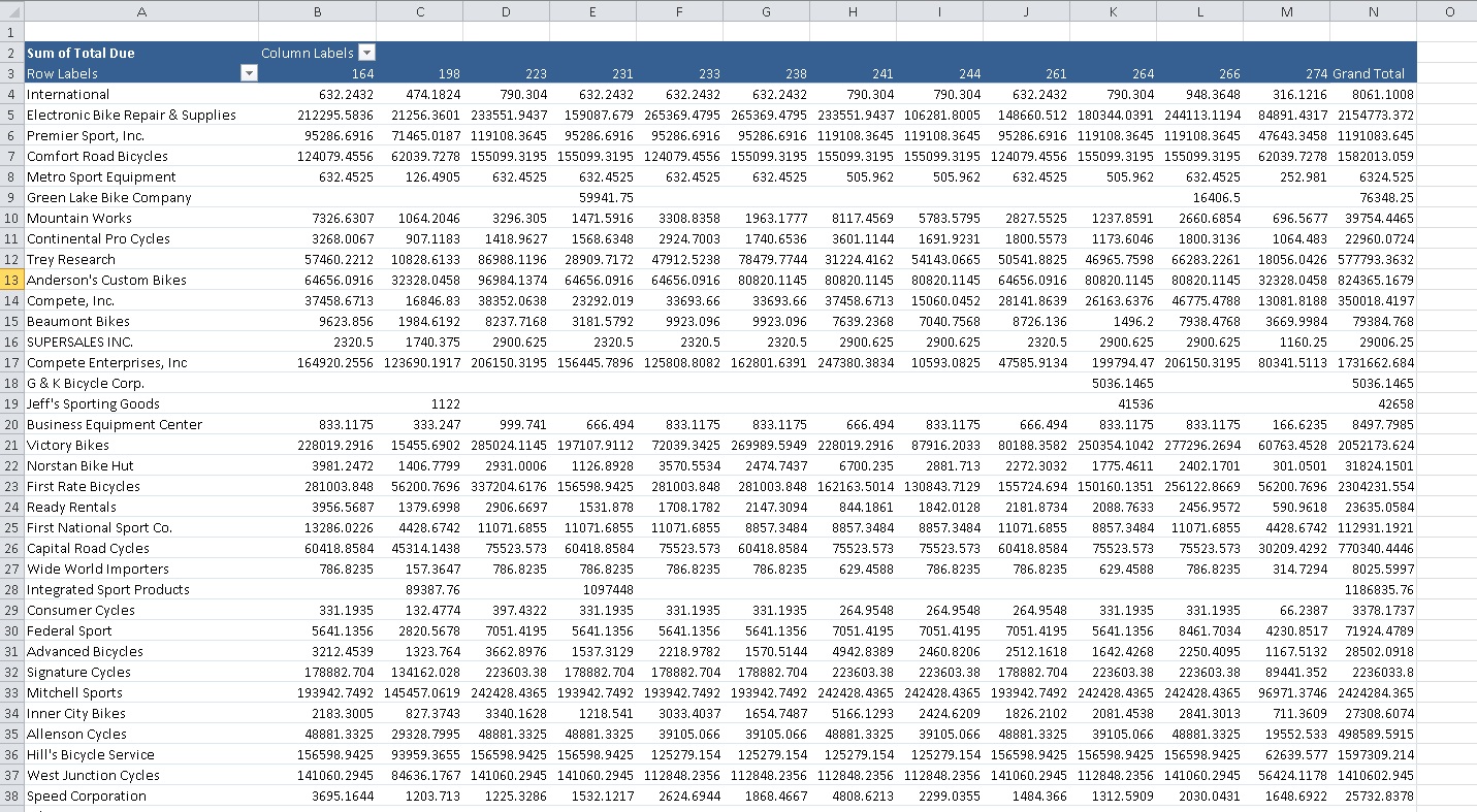 Image Added
Click on the down arrow next to the Vendor Name label. Clear Show All and just select a few vendors.
Image Removed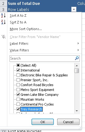 Image Added
Do the same for the EmployeeID field.
Image Removed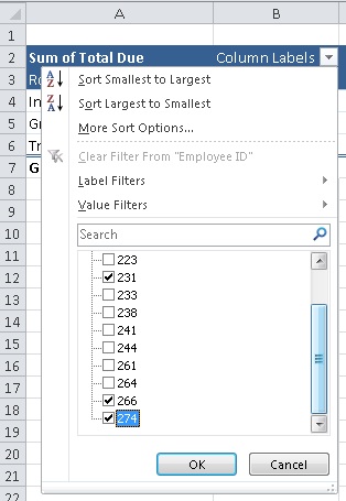 Image Added
Now look at your results.
Image Removed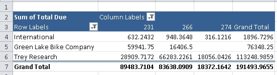 Image Added
Viewing the Report in Reporting Services Report Manager
...
To see the report as you designed it with OfficeWriter:
- From the Select a format export option drop-down list, choose Excel (.xls) designed by Officewriter.
# Click Export.
# You will be prompted to save or open the output file. If your report contains a chart or a PivotTablePivotTable AND you are using Internet Explorer 8 or earlier, you MUST select Save. After it saves to disk, then you may select Open to view it.
This is because of an issue with how Internet Explorer caches temporary internet files. If you are using any other browser or Internet Explorer 9 or later, this issue does not occur and you can open the file directly.
