Templates and PivotTables

A PivotTable report is an interactive table which allows the user to have multiple views of data. By changing the view, the PivotTable report can show different summaries of the data or drill down to display more details for particular areas. ExcelWriter allows you to include PivotTables in an ExcelWriter template file. If there are PivotTables in the original template file, they will be preserved when the template is processed using ExcelWriter.

 

What is a data marker?

An ExcelWriter template is a file created in Microsoft Excel that contains data markers. A *data marker* is a cell value beginning with %%= or %%=$ that specifies a database column, variable, or array to insert in the spreadsheet cell or column containing the marker. ExcelWriter gets values at runtime from a data source and imports them to spreadsheet data markers.

For detailed information on data markers, see Creating Data Markers.

Data markers and PivotTables

ExcelTemplate data markers can be used to bind data to a template for use with a PivotTable. When ExcelTemplate binds the data to the data markers, it also updates the range that the PivotTable uses as a PivotTable cache. By setting the PivotTables to refresh on opening, they will automatically bring in the new values from the PivotTable cache.

How to create and ExcelWriter Template with PivotTables

1. Create a template file containing data markers, each with their own column heading (see [How To Use Templates]). Do not create any of the PivotTables yet.
   

2. Create a pivot table
   

   In Excel 2003: Use Microsoft Excel's _PivotTable and PivotChart Report Wizard_ to create a PivotTable referencing the range of cells containing the column headings and data markers.
   

   In Excel 2007 or above: Use the Ribbon controls (in Excel 2007 and beyond) to create a PivotTable referencing the range of cells containing the column headings and data markers.
    

    

3. Specify the initial layout and field formatting for the PivotTable. Place the PivotTable in any worksheet you desire. (See the Excel documentation for more details about creating your PivotTable.)

4. In Excel 2003: Before clicking "Finish" in the Wizard, click the "Options" button and make sure that "Refresh on open" is checked.
   

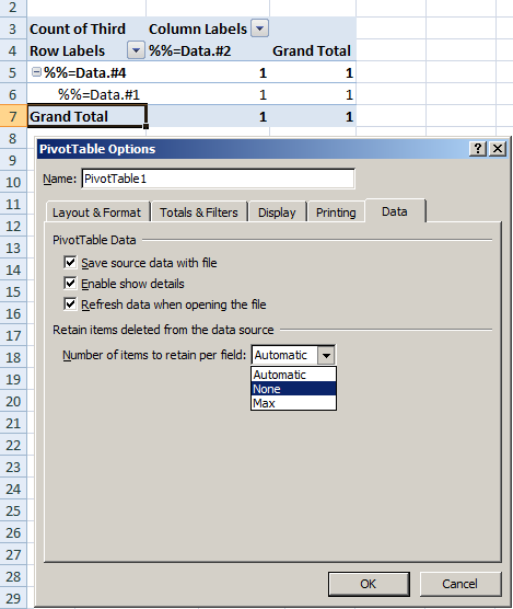
   In Excel 2007 or above: After creating the PivotTable, right-click on the table and select "PivotTable Options". Click on the Data tab and make sure that "Refresh data on opening the file" is checked. Also, make sure to select None from the Number of items to retain per field.
    

    

5. In your newly created PivotTable, you will now see the data markers. Data markers in the PivotTable will be ignored by ExcelWriter, which will instead update the data source.
   
   
   

6.  Repeat steps 2 through 5 for every PivotTable you wish to create. Finish creating your template file and save it in the location on your server which will be accessed by your ExcelWriter script.