
.
This part focuses on adding some Excel formulas to the template file from Part 1. Specifically, this covers adding and formatting a pie chart in the template file. We will only be modifying the template file. There are no changes to the code from Part 2.
1. Open the template file in Excel.
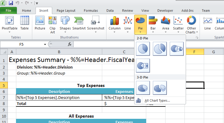
2. Go to the Insert tab on the ribbon. In the Charts group, select a pie chart from the Pie drop-down.
3. Drag the chart to its final position in cell F2.
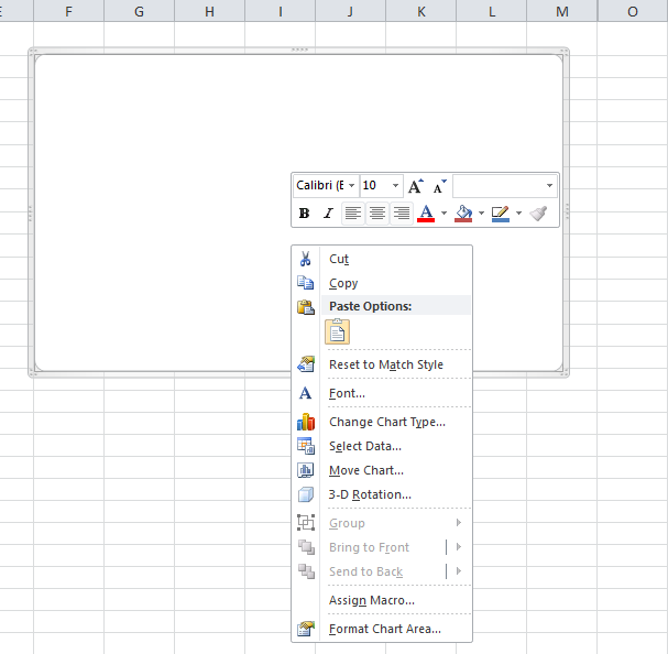
4. Right click on the empty chart and select 'Select Data...' from the menu options.
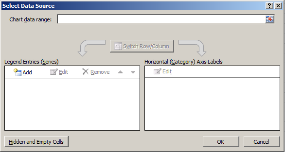
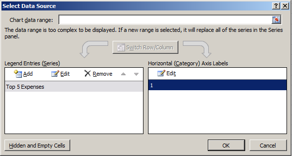
5. In the Select Data Source dialog, under Legend Entries (Series), click Add.
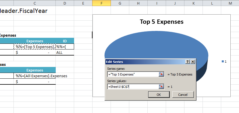
6. In the Edit Series dialog, give the series a name (e.g. "Top 5 Expenses").
7. Click in the Series Values box and then select C5. Then click OK.
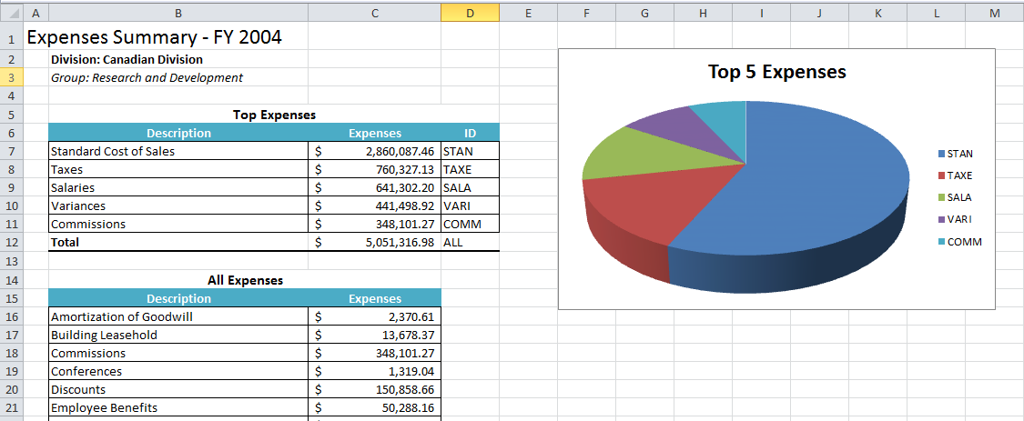
This will put the formula =Sheet1!$C$7 as the formula for the series values. When ExcelWriter inserts data, this formula will expand to include the new rows, so all the top 5 expenses data will be included in the chart series.
8. In the Select Data Source dialog, select the Horizontal (Category) Axis Label that was automatically added and click Edit.
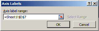
9. In the Axis Labels dialog, click in the Axis label range box if the cursor is not already there. Select D7. Then click OK.
This will put the formula =Sheet1!$D$7 as the formula for the category axis values. In Part 2 we added a formula in D7 to generate 4-charater labels from the Description field in Top Expenses.
10. Once you have returned to the Select Data Source dialog, click OK.
11. Run the report.
You will see that the pie chart is pulling the data from C7:C11 and the labels from D7:Dll.
You can download the code for the Basic ExcelWriter Tutorials as a Visual Studio solution, which includes the Simple Expense Summary.
