.
| Wiki Markupexcerpt |
|---|
When you include a chart in a template spreadsheet, you can use a [ |Creating Data Markers]column as a data source for the chart. Excel will automatically adjust charts to include the number of rows that ExcelWriter assigns to the data marker column. h2. |
...
...
...
...
...
...
[
...
...
]
...
[
...
...
]
In Microsoft Excel, create an ExcelWriter template. For instructions on creating a template, see How to Use Templates.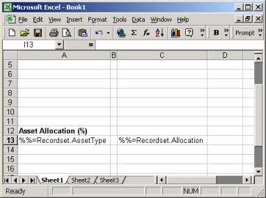
Use Excel's Chart Wizard to create a chart in your spreadsheet. Open the Insert menu and select Chart..., or click the toolbar's Chart Wizard icon. Select the type of chart you would like to create and click Next.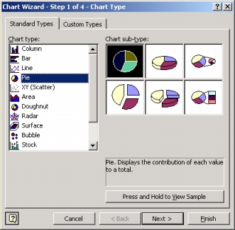
In the Data Range field, enter the cell that contains the data marker that you want to use as a data source for your chart. Excel requires both a starting point and an ending point in the Data Range Field. So, if your data marker is at cell C13, enter =Sheet1\!$C$13:$C$13
...
.
...
The
...
number
...
of
...
rows
...
ExcelWriter
...
will
...
insert
...
at
...
the
...
data
...
marker
...
will
...
vary,
...
and
...
Excel
...
will
...
automatically
...
adjust
...
the
...
chart
...
to
...
include
...
all
...
data
...
in
...
the
...
data
...
marker
...
column.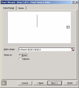
Select the Series tab, and in the Category Label field, enter the range of cells containing the label data marker. Include starting and end points in the category label range. For example, if the label data marker is at cell A13, enter =Sheet1\!$A$13:$A$13
...
and
...
Excel
...
will
...
automatically
...
adjust
...
the
...
chart
...
for
...
the
...
amount
...
of
...
data
...
that
...
fills
...
the
...
spreadsheet.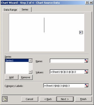
Enter a chart title and click Next.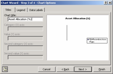
Select a chart location and click Finish to insert the chart into your spreadsheet.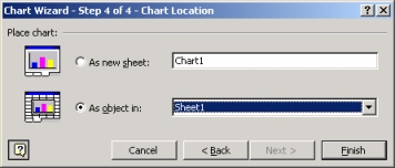
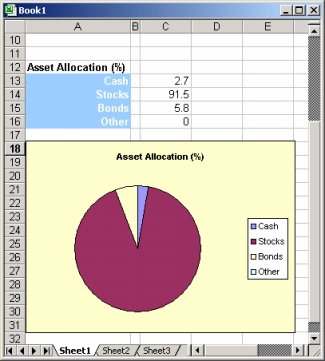
The unpopulated chart is now in your spreadsheet.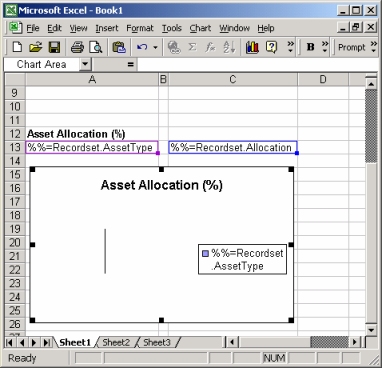
Format the chart and data marker cells as you would like them to appear when the final spreadsheet is created. Data marker formatting is carried down to each inserted cell when data is dynamically entered into the spreadsheet by ExcelWriter.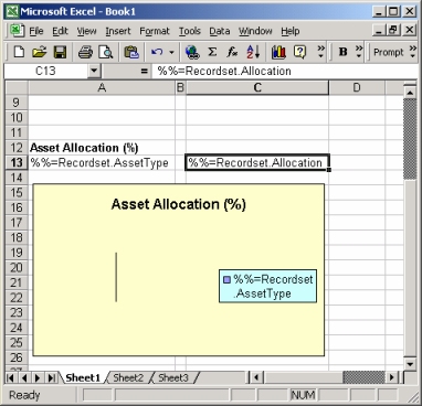
Run your ExcelWriter application to populate the spreadsheet.