
.
Table of Contents |
|---|
This example takes an existing workbook that contains some data and creates a PivotTable. The workbook used in this example is available for download: Download BasicExample.xlsx.
Before writing any PivotTable code, make sure to open the workbook with ExcelApplication and get references to the data worksheet and a worksheet for the PivotTable. See Adding OfficeWriter to your .NET Application.
The data source needs to be a continuous block of cells with a header row with column names. The data source can be defined as an Area or a NamedRange.
Here is a snapshot of the data for this tutorial, which can also be found in BasicExample.xlsx:
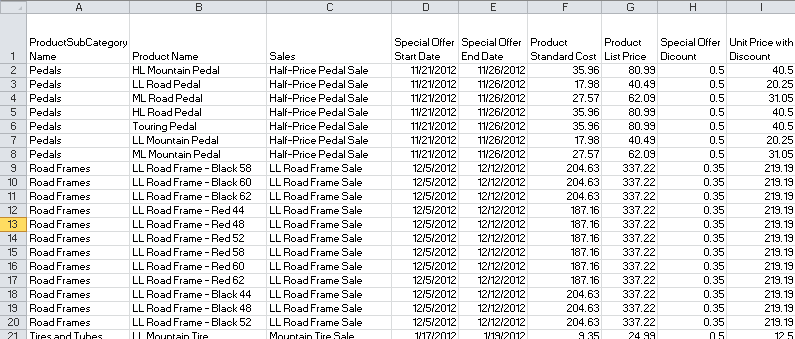
There are 9 columns and 244 rows in the data set, including the row with the header values.
In this case, the data source for the PivotTable will be a dynamically defined area on the data worksheet. Note that the row of column names is included in the area.
To create a PivotTable, call CreatePivotTable on the PivotTables collection. Specify the 0-indexed row and column values for the PivotTable location:
In Excel, there are a number of options that can be set by going to PivotTable Options. These properties are available through PivotTableSettings.
There are a couple properties that you should always consider when working with PivotTables with ExcelWriter.
After creating the PivotTable, always set RefreshOnOpen to true.
ExcelWriter does not have the ability to render a PivotTable, so any modifications made to a PivotTable will not take affect until the output file is opened in Excel and the PivotTable is refreshed. If RefreshOnOpen is true, Excel will refresh the PivotTable when the workbook opens, which will re-render the PivotTable.
The other important property to set is ItemsToRetain. When the PivotTable is created, the values that are available through the row label, column label, or page field drop-down filters are based on the values in the data source of the PivotTable at the time the PivotTable was created.
By default, the PivotTable will retain all the original values in those filters, even if those values are no longer in the data source. Set ItemToRetain to None to make sure the original values are cleared out when the PivotTable is refreshed.
Next, add PivotTableFields to the PivotTable. There are four types of PivotTableField: DataFields, RowLabels, ColumnLabels, and PageFields (or report filters). The Pivot field properties are available for all four types of PivotTableField, however some properties will not have an affect in the output file, depending on the type of field.
All PivotTableFields are created from SourceFields. A SourceField is a read-only field that is automatically generated from the data source of the PivotTable. Each column in the data source corresponds with a SourceField in the PivotTable and the name of the SourceField comes from the column header name.
To add a PageField, call CreateField on the PivotTable.PageFields collection. You will need to specify the SourceField that will be used to create the PageField.
Similarly to page fields, RowLabels and ColumnLabels are created on the PivotTable.RowLabels and PivotTable.ColumnLabels collections. As mentioned earlier, only one RowLabel, ColumnLabel, or PageField can be created from a particular SourceField.
Excel automatically sorts and re-renders a PivotTable any time a change is made. By default, the row label or column label values are sorted alpha-numerically in ascending order.
Since ExcelWriter does not have the ability to render PivotTables or sort the values for a field, the only way to guarantee that the data will be sorted is to set RefreshOnOpen to true and set SortOptions.Ordering on a PivotTablefield to be Ascending or Descending.
This property only affects row and column labels.
When Excel refreshes the PivotTable, it will observe the SortOptions setting for a particular field.
Adding data fields - calculated fields, naming conventions, changing the display name
To create a data field, call CreateField on the DataFields collection. Unlike row labels, column labels, and page fields, multiple data fields can be created from the same source field.
In Excel, a unique name is given to the data field depending on the type of data in the source field (numerical or mixed), whether or not any other data fields were already created from the same source field, and whether the source field name ends in a number or alphabetical character (e.g. Case1 vs. CaseOne).
ExcelWriter uses a consistent naming convention when creating data fields: all data fields follow the format SOURCEFIELDNAME_#, where # is an incremental number starting at 1. To change the name of a data field, use the DisplayName property.
And that concludes how to create a basic PivotTable. Here is the full sample code below:
