
.
Table of Contents |
|---|
This part focuses on adding some Excel formulas to the template file from Part 1. Specifically, this covers combining data marker values with other text, adding a 'Total' row after imported data, and including formulas in imported data rows.
Since the formulas are native Excel functionality, we will only be modifying the template file. There are no changes to the code from Part 1.
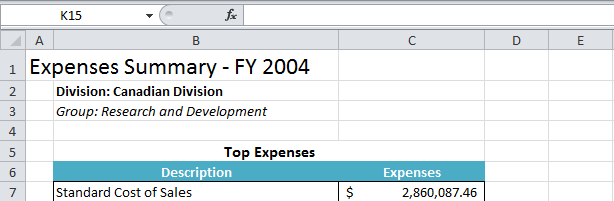
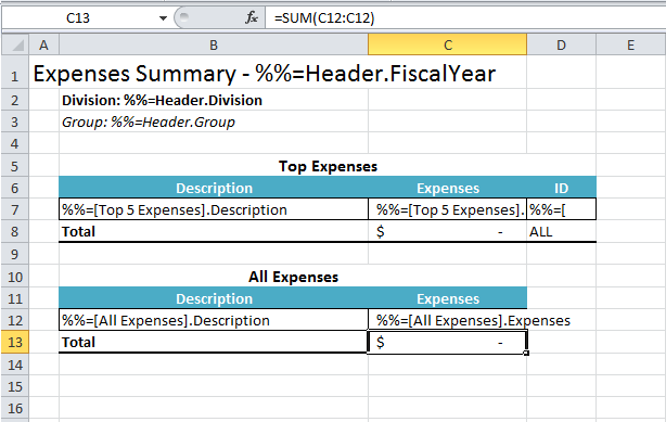
We start with the template file as it was at the end of Part 1:
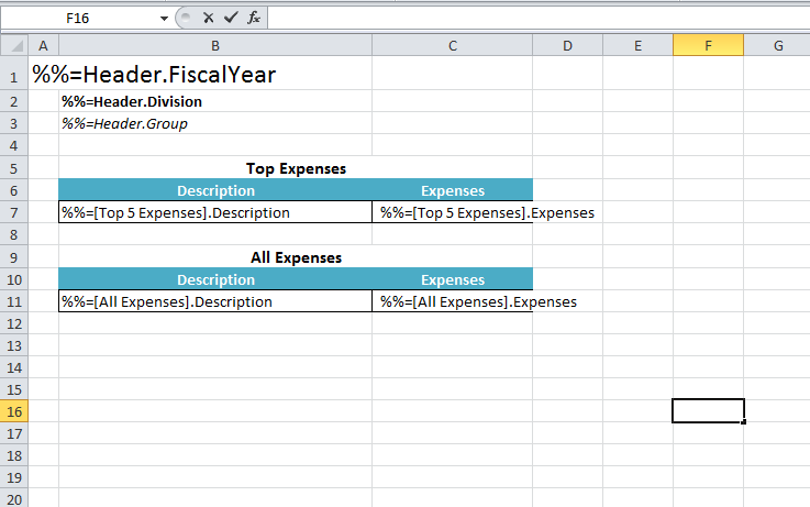
Right now, the header is set up just to display the values for FiscalYear, Division, and Group. Let's say we want to change the labels to "Expenses Summary - <Fiscal Year>", "Division: <Division>", "Group: <Group>". Data markers must be the only content a cell, they cannot be combined with other text. To get around this, you need to build the text or formula with a reference to the cell the data marker occupies.
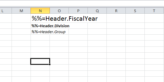
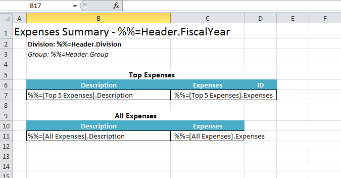
1. Move the data markers for %%=Header.FiscalYear, %%=Header.Division, %%=Header.Group to a column off to the right, say Column N.
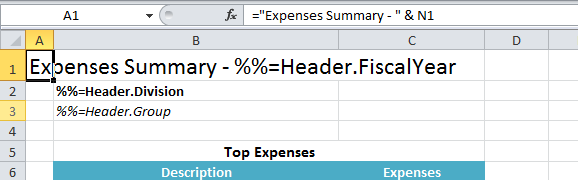
2. In A1, replace %%=Header.FiscalYear with a formula that builds the desired string with the formula ="Expenses Summary - " & N1.
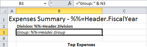
3. In B2 and B3, replace %%=Header.Division and %%=Header.Group with similar formulas: ="Division: " & N2, ="Group: " & N3.
4. Hide column N so the extra data markers won't be visible.
5. Run the code.
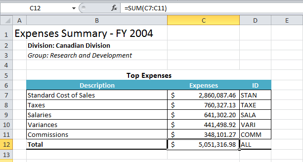
In the output you will see the text combined with the values of the data markers:
If a formula references a data marker row, ExcelWriter will update the formula to reflect that multiple rows are being inserted. In this section, we'll briefly cover how ExcelWriter handles formulas that are on the data marker row.
Let's say we want to generate some short labels for the Top 5 Expenses to use with the descriptions. One possibility is to add the labels to the data source (i.e. through the SQL query or modifying the data structure directly), but another way is to use Excel formulas.
Similar to the last section, we'll use the existing data markers to create a new string for the Top 5 Expenses table.
6. In Column D, create a header for the label. Update the 'Top Expenses' merged cell area to include column D.
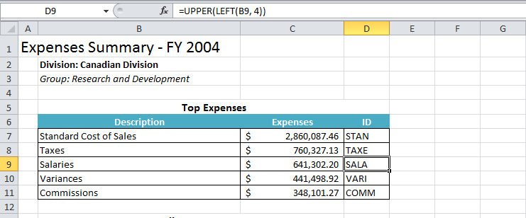
7. In cell D7, add a formula =UPPER(LEFT(B7, 4)).
Excel's LEFT(text, N) function returns the first N characters from the text, starting from the left. In this case, the first 4 characters from cell B7. Then the UPPER function converts the characters to uppercase.
ExcelWriter will update this formula for each row of data that is added, so the formula in row 9 will read =UPPER(LEFT(B9, 4)).
8. Run the report.
You will see that the first 4 characters from the description have been set to uppercase in column D.
If an aggregate formula, such as TOTAL or SUM, references a data marker row, ExcelWriter will stretch the formula to include all the rows that have been inserted. In this section, we'll cover how to add a total row.
9. Insert a new row below Top Expenses and All Expenses. Add labels for the total row and format as desired.
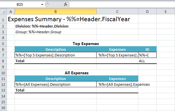
10. In cell C8, add the formula =SUM(C7:C7). Add a similar formula to C13: =SUM(C12:C12). Don't forget to format C8 and C13 to use currency formatting.
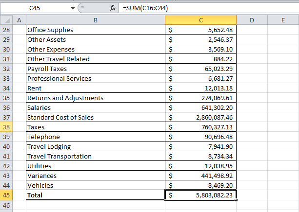
When ExcelWriter imports the data, the first formula will get stretched to C7:C11. The second formula will first get updated to account for the new data inserted above it (C16:C16) and then will get stretched to C16:C44.
11. Run the report.
You will see that the formulas have been stretched and updated as described above.
You can download the code for the Basic ExcelWriter Tutorials as a Visual Studio solution, which includes the Simple Expense Summary.

