You are viewing an old version of this page. View the current version.
Compare with Current
View Page History
Version 1
Next »
Excel charts can play an important part in data presentation. The ability to visually present data is one of Excel's strong points. This section shows you how to include Excel charts in the reports you create with OfficeWriter Designer. Each time you execute your report, the chart will be populated with the most recent data.
Creating a Chart
The source data for an Excel chart is a range of cell values. But, OfficeWriter Designer places data markers in your worksheet which are later populated with a set of values from a database. How do you specify that the database values should be used as the source data for a chart series? In Excel's Chart Wizard, set the source data to be the cell that contains the data marker, but specify the cell as a range, not as an individual cell address. For example, use =Sheet1!$B$2:$B$2 instead of =Sheet1!$B$2
- Open Microsoft Excel, click Add Query on the OfficeWriter toolbar, and create the following query.
This query returns the sales from the AdventureWorks database broken down by Product Category.
# Using OfficeWriter's Insert Field button, insert the fields in the worksheet, as shown:
!xlw_eChart1.jpg!
# From the Excel's Insert menu, select Chart. The Chart Wizard will open.
# Select the chart type Exploded pie with a 3-D visual effect.
!xlw_eChart2.jpg!
# Click Next.
# Select the Series tab.
!xlw_eChart3.jpg!
# Click Add add a series.
# In the Values text box, enter the address of the cell containing the query's Total field, but enter it as a range, not as an individual cell address: *=Sheet1!$B$2:$B$2*
!xlw_eChart7.jpg!
\OfficeWriter will take this range and populate it with the query's data. If you click the icon to the right of the Values box and select the cell with your mouse, your cell will be selected, but not as a range.
!xlw_eChart4.jpg!
\Add :$B$2 to make sure the cell is selected as a range.
!xlw_eChart5.jpg!
- Do the same for the cell containing the query's Category field.
!xlw_eChart6.jpg!
# Click Next.
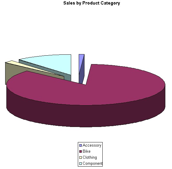
# In the Chart Title textbox, enter Sales by Product Category, and click Next.
!xlw_eChart8.jpg!
# In the Chart Location dialog, select either As new sheet or As object in, and click Finish.
Viewing the Chart
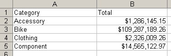
Publish and View your report and chart. The data from the query will look like this:
The chart should look like this: